Sunday Reading Notes series is back : Let’s understand the magical rule of ‘tuning your MH algorithm so that the acceptance rate is roughly 25%’ together!
‘Tune your MH algorithm so that the acceptance rate is roughly 25%’ has been general advice given to students in Bayesian statistics classes. It has been almost 4 years since I first read about it from the book Bayesian Data Analysis, but I never read the original paper where this result first appeared. This Christmas, I decided to read the paper ‘Weak Convergence and Optimal Scaling of Random Walk Metropolis Algorithms’ by Roberts, Gelman and Gilks and to resume by Sunday Reading Notes series with a short exposition of this paper.
In Roberts, Gelman and Gilk (1997), the authors obtain a weak convergence result for the sequence of algorithms targeting the sequence of distributions  converging to a Langevin diffusion. The asymptotic optimal scaling problem becomes a matter optimizing the speed of the Langevin diffusion, and it is related to the asymptotic acceptance rate of proposed moves.
A one-sentence summary of the paper would be
if you have a d-dimensional target that is independent in each coordinate, then choose the step size of random walk kernel to be 2.38 / sqrt(d) or tune your acceptance rate to be around 1/4.
Unfortunately, in practice the ‘if’ condition is often overlooked and people are tuning the acceptance rate to be 0.25 as long as the proposal is random walk, no matter what the target distribution is. It has been 20 years since the publication of the 0.234 result and we are witnessing the use of MCMC algorithms on more complicated target distributions, for example parameter inference for state-space models. I feel that this is good time that we revisit and appreciate the classical results while re-educating ourselves on their limitations.
Reference:
Roberts, G. O., Gelman, A., & Gilks, W. R. (1997). Weak convergence and optimal scaling of random walk Metropolis algorithms. The annals of applied probability, 7(1), 110-120.
——–TECHNICAL EXPOSITION——-
Assumption 1 The marginal density of each component  is such that
  is Lipschitz continuous and
![\displaystyle \mathbb{E}_f\left[\left(\frac{f'(X)}{f(X)}\right)^8\right] = M < \infty, \ \ \ \ \ (1)](https://s0.wp.com/latex.php?latex=%5Cdisplaystyle+%5Cmathbb%7BE%7D_f%5Cleft%5B%5Cleft%28%5Cfrac%7Bf%27%28X%29%7D%7Bf%28X%29%7D%5Cright%29%5E8%5Cright%5D+%3D+M+%3C+%5Cinfty%2C+%5C+%5C+%5C+%5C+%5C+%281%29&bg=ffffff&fg=000000&s=0&c=20201002)
![\displaystyle \mathbb{E}_f\left[\left(\frac{f''(X)}{f(X)}\right)^4\right] < \infty. \ \ \ \ \ (2)](https://s0.wp.com/latex.php?latex=%5Cdisplaystyle+%5Cmathbb%7BE%7D_f%5Cleft%5B%5Cleft%28%5Cfrac%7Bf%27%27%28X%29%7D%7Bf%28X%29%7D%5Cright%29%5E4%5Cright%5D+%3C+%5Cinfty.+%5C+%5C+%5C+%5C+%5C+%282%29&bg=ffffff&fg=000000&s=0&c=20201002)
Roberts et al. (1997) considers random walk proposal  where
where  We use
  to denote the Markov chain and define another Markov process
  with
with ![{Z_t^d = X_{[dt]}^d}](https://s0.wp.com/latex.php?latex=%7BZ_t%5Ed+%3D+X_%7B%5Bdt%5D%7D%5Ed%7D&bg=ffffff&fg=000000&s=0&c=20201002) , which is the speed-up version of
, which is the speed-up version of  . Let
. Let ![{[a]}](https://s0.wp.com/latex.php?latex=%7B%5Ba%5D%7D&bg=ffffff&fg=000000&s=0&c=20201002) denote the floor of
denote the floor of  . Define
 ![{U^d_t= X^d_{[dt],1}}](https://s0.wp.com/latex.php?latex=%7BU%5Ed_t%3D+X%5Ed_%7B%5Bdt%5D%2C1%7D%7D&bg=ffffff&fg=000000&s=0&c=20201002) , the first component of
, the first component of ![{X_{[dt]}^d = Z^d_t}](https://s0.wp.com/latex.php?latex=%7BX_%7B%5Bdt%5D%7D%5Ed+%3D+Z%5Ed_t%7D&bg=ffffff&fg=000000&s=0&c=20201002) .
.
Theorem 1 (diffusion limit of first component) Suppose  is positive and in
  and that (1)-(2) hold. Let
  be such that all components are distributed according to and assume
  for all
  . Then as
  ,
,

The  and
and  satisfies the Langevin SDE
and

with  being the standard normal cdf and
![\displaystyle I = \mathbb{E}_f\left[\left(f'(X)/ f(X)\right)^2\right].](https://s0.wp.com/latex.php?latex=%5Cdisplaystyle+I+%3D+%5Cmathbb%7BE%7D_f%5Cleft%5B%5Cleft%28f%27%28X%29%2F+f%28X%29%5Cright%29%5E2%5Cright%5D.+&bg=ffffff&fg=000000&s=0&c=20201002)
Here  is the speed measure of the diffusion process and the `most efficient’ asymptotic diffusion has the largest speed measure.
  measures the `roughness’ of .
Example 1 If is normal, then 
![\displaystyle I = \mathbb{E}_f\left[\left(f'(x) / f(x) \right)^2\right] = (\sigma_f)^{-4}\mathbb{E}_f\left[x^2\right] = 1/\sigma^2_f.](https://s0.wp.com/latex.php?latex=%5Cdisplaystyle+I+%3D+%5Cmathbb%7BE%7D_f%5Cleft%5B%5Cleft%28f%27%28x%29+%2F+f%28x%29+%5Cright%29%5E2%5Cright%5D+%3D+%28%5Csigma_f%29%5E%7B-4%7D%5Cmathbb%7BE%7D_f%5Cleft%5Bx%5E2%5Cright%5D+%3D+1%2F%5Csigma%5E2_f.&bg=ffffff&fg=000000&s=0&c=20201002)
So when the target density is normal, then the optimal value of  is scaled by
  , which coincides with the standard deviation of .
Proof: (of Theorem 1.1) This is a proof sketch. The strategy is to prove that the generator of  , defined by
![\displaystyle G_n V(x^n) = n \mathbb{E}\left[\left(V(Y^n) - V(x^n)\right) \left( 1 \wedge \frac{\pi_n(Y^n)}{\pi_n(x^n)}\right)\right].](https://s0.wp.com/latex.php?latex=%5Cdisplaystyle+G_n+V%28x%5En%29+%3D+n+%5Cmathbb%7BE%7D%5Cleft%5B%5Cleft%28V%28Y%5En%29+-+V%28x%5En%29%5Cright%29+%5Cleft%28+1+%5Cwedge+%5Cfrac%7B%5Cpi_n%28Y%5En%29%7D%7B%5Cpi_n%28x%5En%29%7D%5Cright%29%5Cright%5D.+&bg=ffffff&fg=000000&s=0&c=20201002)
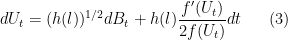
converges to the generator of the limiting Langevin diffusion, defined by
![\displaystyle GV(x) = h(l) \left[\frac{1}{2} V''(x) + \frac{1}{2} \frac{d}{dx}(\log f)(x) V'(x)\right].](https://s0.wp.com/latex.php?latex=%5Cdisplaystyle+GV%28x%29+%3D+h%28l%29+%5Cleft%5B%5Cfrac%7B1%7D%7B2%7D+V%27%27%28x%29+%2B+%5Cfrac%7B1%7D%7B2%7D+%5Cfrac%7Bd%7D%7Bdx%7D%28%5Clog+f%29%28x%29+V%27%28x%29%5Cright%5D.+&bg=ffffff&fg=000000&s=0&c=20201002)
Here the function  is a function of the first component only.
First define a set

where
![\displaystyle R_d(x_2,\ldots,x_d) = (d-1)^{-1} \sum_{i=2}^d \left[(\log f(x_i))'\right]^2](https://s0.wp.com/latex.php?latex=%5Cdisplaystyle+R_d%28x_2%2C%5Cldots%2Cx_d%29+%3D+%28d-1%29%5E%7B-1%7D+%5Csum_%7Bi%3D2%7D%5Ed+%5Cleft%5B%28%5Clog+f%28x_i%29%29%27%5Cright%5D%5E2+&bg=ffffff&fg=000000&s=0&c=20201002)
and
![\displaystyle S_d(x_2,\ldots,x_d) = - (d-1)^{-1} \sum_{i=2}^d \left[(\log f(x_i))''\right].](https://s0.wp.com/latex.php?latex=%5Cdisplaystyle+S_d%28x_2%2C%5Cldots%2Cx_d%29+%3D+-+%28d-1%29%5E%7B-1%7D+%5Csum_%7Bi%3D2%7D%5Ed+%5Cleft%5B%28%5Clog+f%28x_i%29%29%27%27%5Cright%5D.+&bg=ffffff&fg=000000&s=0&c=20201002)
For fixed  , one can show that
  goes to 1 as . On these sets
  , we have

which essentially says  , because we have uniform convergence for vectors contained in a set of limiting probability 1.

Corollary 2 (heuristics for RWMH) Let

be the average acceptance rate of the random walk MH in  dimensions.
We must have  where
where  .
.
is maximized by  and
and  and
and 
The authors consider two extensions of the target density  , where the convergence and optimal scaling properties will still hold. The first extension concerns the case where
  ‘s are different, but there is an law of large numbers on these density functions. Another extension concerns the case
  , with some conditions on
  .
.


![\displaystyle \mathbb{E}(p \| q) = \mathbb{E}_{p(z \mid x)} \left[ \log \frac{p(z \mid x)}{q(z ; \lambda)} \right].](https://s0.wp.com/latex.php?latex=%5Cdisplaystyle+%5Cmathbb%7BE%7D%28p+%5C%7C+q%29+%3D+%5Cmathbb%7BE%7D_%7Bp%28z+%5Cmid+x%29%7D+%5Cleft%5B+%5Clog+%5Cfrac%7Bp%28z+%5Cmid+x%29%7D%7Bq%28z+%3B+%5Clambda%29%7D+%5Cright%5D.&bg=ffffff&fg=000000&s=0&c=20201002)

![{L_{\mathrm{KL}} = \mathbb{E}_{p(z \mid )}[ - \log q(z ; \lambda)],}](https://s0.wp.com/latex.php?latex=%7BL_%7B%5Cmathrm%7BKL%7D%7D+%3D+%5Cmathbb%7BE%7D_%7Bp%28z+%5Cmid+%29%7D%5B+-+%5Clog+q%28z+%3B+%5Clambda%29%5D%2C%7D&bg=ffffff&fg=000000&s=0&c=20201002)
![\displaystyle g_{\mathrm{KL}}(\lambda) := \nabla L_{KL}(\lambda) = \mathbb{E}_{p(z \mid x)}\left[- \nabla_{\lambda} \log q(z; \lambda)\right].](https://s0.wp.com/latex.php?latex=%5Cdisplaystyle+g_%7B%5Cmathrm%7BKL%7D%7D%28%5Clambda%29+%3A%3D+%5Cnabla+L_%7BKL%7D%28%5Clambda%29+%3D+%5Cmathbb%7BE%7D_%7Bp%28z+%5Cmid+x%29%7D%5Cleft%5B-+%5Cnabla_%7B%5Clambda%7D+%5Clog+q%28z%3B+%5Clambda%29%5Cright%5D.&bg=ffffff&fg=000000&s=0&c=20201002)


 number of held-out test sets and each set has some predictive score when the rest of the data is used for training. The leave-
 , is the average of these predictive scores. When the log posterior predictive probability is used as the scoring rule, then we must have

 of the reward function
  -eluder dimension, which is a measure of complexity of a set of functions. An action
  is independent of actions
  with respect to
  . Being a Bayesian statistician, I am naturally curious about the ‘miss-specified’ case. Will the regret bound decompose in terms of distance from
  . Unlike random walk Metropolis algorithm, in MALA, the proposal distribution uses the gradient of
  at
at  :
:
 is the step variance and
  is a d-dimensional standard normal. Following this proposal, we perform an accept / reject step, so that the resulting Markov chain has the desired stationary distribution:
 : absolute value of the first 8 order derivatives are bounded,
  is Lipschitz, and all moments exist for
  starting from stationarity and following the MALA algorithm with variance
  for some
  . Let
. Let  be a Poisson process with rate
  ,
,  and
and  is the first component of
  , i.e.
  . We must have, as
  , where
 is the speed measure and
 ![{K = \sqrt{\mathbb{E} \left[\frac{5g'''(X)^3 - 3g''(X)}{48}\right]} > 0}](https://s0.wp.com/latex.php?latex=%7BK+%3D+%5Csqrt%7B%5Cmathbb%7BE%7D+%5Cleft%5B%5Cfrac%7B5g%27%27%27%28X%29%5E3+-+3g%27%27%28X%29%7D%7B48%7D%5Cright%5D%7D+%3E+0%7D&bg=ffffff&fg=000000&s=0&c=20201002) .
. such that
  and on these sets the generators converges uniformly.
 where
where 
 . Also the step variance should be tuned to be
 of RWM. But let’s also keep in mind that MALA requires an extra step to compute the gradients
  , which takes